Late interaction under the microscope
Multi-vector Search A field guide to keeping local evidence alive , matching it precisely, and shipping it at production scale.
Query tokens
auth
credentials
Local match 0.94
Keep the clue. Score it late.
I am Amélie Chatelain, a senior machine learning engineer at LightOn and head of training and inference; my PhD is in physics. LightOn builds search infrastructure for AI agents, so much of our machine-learning work is information-retrieval centric.
This field guide was created as the guest lecture on late interaction and multi-vector search for the 22 July 2026 cohort of AI-Powered Search: Modern Retrieval for Humans & Agents, hosted by Trey Grainger and Doug Turnbull. The cohort had already introduced single-vector, sparse and dense retrieval and the MaxSim operator; this session puts that one retrieval shape under the microscope.
The goal is practical: understand where one pooled vector loses evidence, how late interaction preserves it, where a cross-encoder still belongs, and which production techniques make the richer representation workable.
Late interaction under the microscope
Single-vector dense search uses one fixed-size embedding for the query and for each indexed unit / document.
query q
q1 q2 q3 q4
Encoder
pool
one vector
document d
d1 d2 d3
d4 d5 d6
Encoder
pool
one vector
What becomes possible when every token or patch gets a voice?
Before we zoom in, let me quickly reset the baseline: in single-vector dense retrieval, the query is one fixed-length vector, and each indexed unit (usually a passage or chunk) is also one vector. The two sides are encoded independently, so the indexed vectors can be prepared offline. At search time we rank with a similarity score, usually via an ANN index.
This is fast and scalable. But it makes one strong bet: that a single representation has preserved every clue a future query might care about. The rest of the guide examines what happens when that bet fails, and when keeping multiple local vectors is worth the extra cost.
So, if single-vector search is this efficient, why does Claude Code still reach for grep?
Why does Claude Codegrep ?
If we have strong language models and strong embedding models,
$ grep -rn "refresh_token" auth/
Let's start with a puzzle. With the release of Claude Code, we've seen a resurgence of "Grep is all you need" across coding agents, but why?
If we have very capable language models and increasingly strong embedding models, why would a frontier coding agent still reach for a line-oriented tool whose roots go back to the 1970s? Let the question sit for a moment: grep's persistence is evidence about the retrieval job, not merely nostalgia.
Grep is hard to beat, and not only for infra
The boring infra reasons
Zero infra: works on any machine.No model to deploy.No index to maintain.Privacy by default.
But also: why it sticks
Lexical matching is extremely strong for code .
Granularity is non-negotiable: exact symbols, paths, functions & error strings matter.Code is very formatted data , which grep can exploit.
The bar for a learned retriever: earn its keep by adding semantics without losing exact local clues .
The infra answer is completely real: grep is local, cheap, private, runs on almost any toaster, and requires no model or index service.
But on top of that, for code, lexical matching is very strong. Code is very formatted compared to regular text, which grep can exploit; and in code granularity is essential: exact function names, error codes, and so on. That is built-in with lexical search. So the bar for a dense retriever to justify the extra hassle of deployment plus index maintenance is high: it needs to keep this granularity while adding semantics.
One underappreciated part of the bargain is retries: an agent can cheaply brute-force several reformulations through grep until one lands. Even a limited retriever becomes "good enough" when iteration is almost free. Anthropic has mentioned internal benchmarking, but without a published controlled comparison the strongest defensible explanation is this combination of exactness, locality, zero deployment cost and cheap retries.
Single-vector search compresses every clue into one summary
One query can carry many independent relevance clues : protocol terms, a status code, a function name, a file path.
A single vector of dimension d must compress every clue into one fixed-size object.
"What's the backoff for OAuth token refreshes after a 429 ?"
RetryPolicy
HTTP 429
refresh_token()
auth/session.py
↓
[ single vector · dim d ]
→ diluted signal
Look at how many independent clues are packed into this one example query: OAuth, a retry policy, HTTP 429, a function-shaped term, and a likely file path. This isn't just "a semantic question about authentication."
A single dense vector has to carry every one of those constraints in one fixed-size object. That compression is the bottleneck to remember throughout the deck: one pooled vector must decide what to preserve before it knows which detail the future query will care about.
Just increase the dimension? … well… introducing LIMIT!
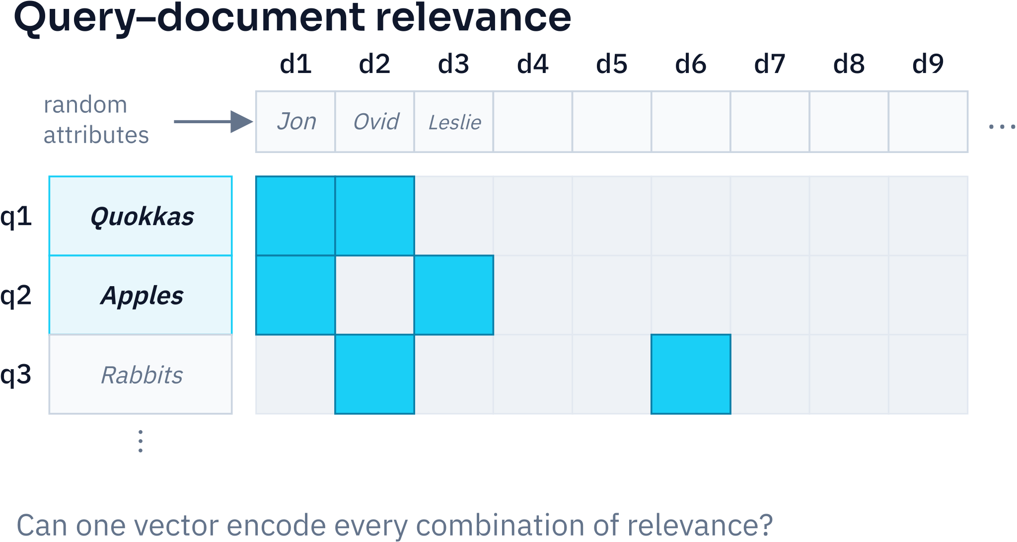
The construction of the dataset: can one vector encode every combination of relevance?
A toy dataset, yes, but also similar to product queries :gaming monitor 27" 140Hz
On the Theoretical Limitations of Embedding-Based Retrieval · Weller et al. · ICLR 2026
Your first instinct may be: if the vector is too compressed, make it bigger and problem solved, no?
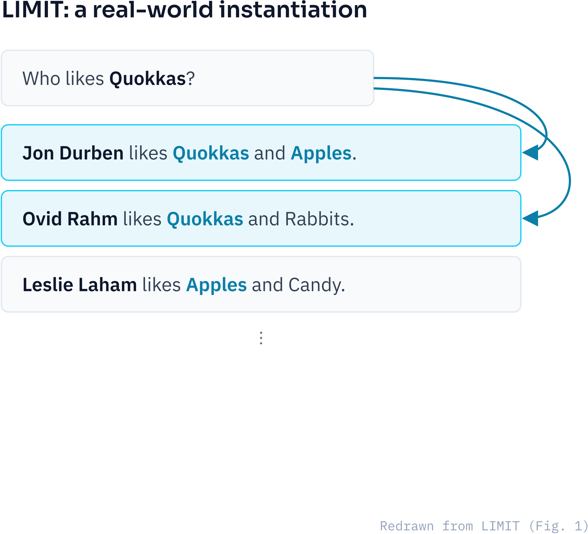
LIMIT gives a clean way to see why that doesn't fully solve the structural problem. The paper first shows mathematically that there is a limit to how much data can be encoded in a single vector. What I want to show you is their toy dataset: random attributes (Quokkas, Apples...) and people's names; each document contains combinations, and queries ask for them.
It was designed as an example of dense-model limitations, but product search has the same shape: "27-inch gaming monitor, 140 hertz" is not one vague intent but several constraints that must all survive.
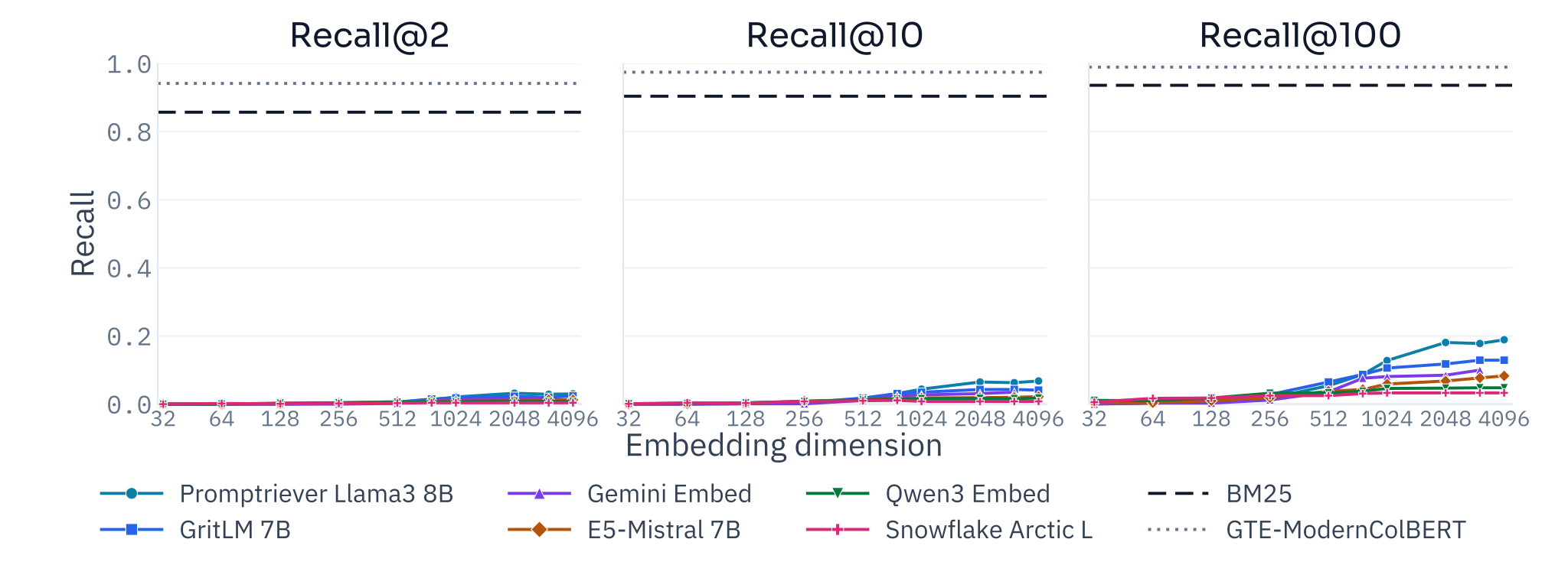
Bigger vectors plateau
Increasing the dimension helps… to a point. It does not change the structure of the problem.
Even a simple retrieval setting can expose a ceiling .
More capacity ≠ preserving local evidence .
Large d becomes impractical at corpus scale.
What they find on this benchmark: as the embedding dimension increases, the dense models improve a little, but they stay far below the lexical reference. And most importantly, there seems to be a plateau.
Capacity and structure are not the same thing. Making a single vector bigger gives it more room, but it does not preserve local evidence the way keeping multiple vectors does. The paper stops at 4K dimensions; beyond the plateau, serving 8K- or 16K-dimensional embeddings across a large corpus becomes its own memory and compute problem. "Just keep increasing d" is not a satisfying escape route.
No! Exact match is a gift, but it's sparse
Vocabulary mismatch is alive and well: lexical search breaks the moment the user says auth and the code says credentials .
→ We need exact granularity and semantic matching.
Now, the wrong conclusion would be that grep or BM25 is all we need. Exact match is incredibly strong when the vocabulary lines up, but vocabulary mismatch is everywhere.
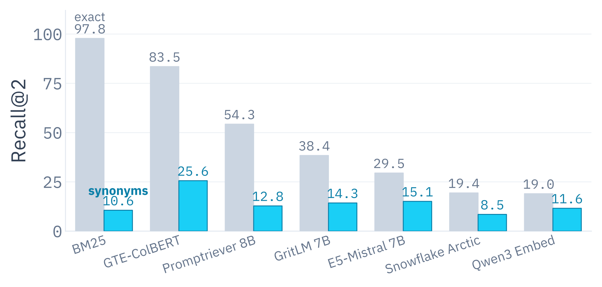
LIMIT has a synonym version where they replaced the corpus items by synonyms, and as you'd expect, BM25 drops terribly.
A user says "auth" while the code says "credentials": lexical retrieval gives granularity, but not enough semantic flexibility. We want exact-ish local evidence and soft semantic matching at the same time.
But wait…
There's one line on this chart that doesn't behave like the ordinary dense models: GTE-ModernColBERT. Is it a bird, is it a plane? It is not solving the problem by making one pooled embedding enormous. It uses a different retrieval paradigm: late interaction.
So rather than asking how to squeeze more into one vector, let's ask what happens if we keep multiple local vectors and delay their interaction until the query arrives.
Late interaction sits in the middle
← cheaper · more scalable more accurate · expensive →
Single-vector Retrieval Pooled dual encoder
document d
d1 d2 d3 d4 d5 d6
Encoder
docs encoded offline
document d
d1 d2 d3 d4 d5 d6
Encoder
docs encoded offline
Full-interaction reranking Cross-encoder
ColBERT: Efficient and Effective Passage Search via Contextualized Late Interaction over BERT · Khattab et al., 2020
Consider an axis ranking retrieval methods from cheap and scalable to accurate but expensive.
On the left, our trusty pooled bi-encoder powering single-vector retrieval: queries and documents each go separately through an encoder, and the produced vectors are pooled into a single vector. Cheap, because the document side can be prepared offline.
On the right, a cross-encoder lets query and document tokens interact deeply: our most powerful way to do retrieval, but that work happens for every candidate at query time.
Late interaction sits in the middle: encode as in the single-vector setup, but don't pool; DELAY the interaction. It keeps the offline document encoding of a bi-encoder, but lets the query interact with local document vectors during scoring.
Reintroducing MaxSim
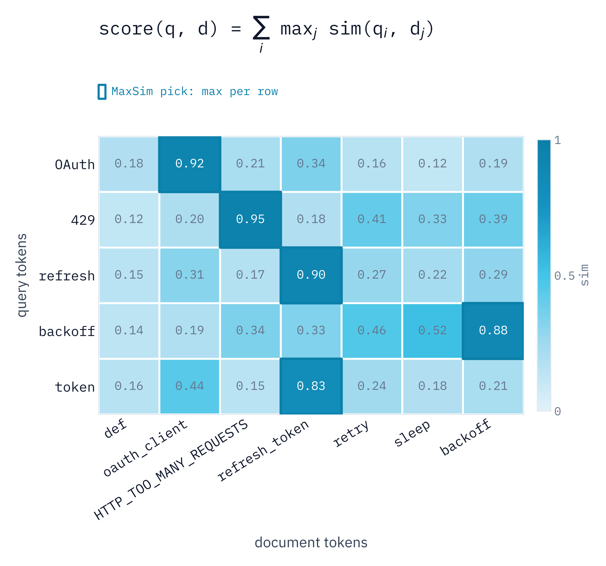
score(q, d) = Σ i max j sim(qi , dj )
For every query token , find its best-matching document token, then sum those best matches.
max keeps rare, high-signal evidence from being averaged away.Σ rewards coverage of query evidence by the document.
MaxSim pick: max per row · illustrative similarities
The way these query and document vectors interact is through MaxSim: for every query token, find the best matching token in the document, then add those best matches.
Read the heatmap row by row: each row is a query token, each column a document token, every cell a similarity. For each query token, MaxSim keeps only the best document-side match, then sums those maxima.
Max preserves rare signal: with mean interaction, a token like OAuth would not contribute as much as it should. The sum rewards coverage: a good document should have strong evidence for several parts of the query, not one lucky match. Note it is directional: does the document cover the query's evidence?
What's coming
Lexical
Exact granularity
Dense
Soft semantic matching
The guide starts with two field cases:
01
Code retrieval granularity made impossible to ignore
02
Multimodal retrieval compression made impossible to ignore
Then the production objections: storage · latency · ecosystem .
Multi-vector search has a very useful overlap: lexical search preserves exact local clues, dense search provides soft semantic matching, and late interaction tries to keep both.
We'll make the idea concrete through two field cases: code retrieval makes granularity impossible to ignore; multimodal document retrieval makes compression impossible to ignore. After that, the production objections: storage, latency, updates, and the model ecosystem.
01 FIELD CASE
Code retrieval
Let's begin with code. It's a great stress test because tiny local details often decide relevance, while the user's intent may still be expressed in natural language. Code needs both sides of the story: exact symbols and semantic intent.
Why is code search hard?
Before an agent can fix anything, it has to find the files and lines that matter. And code is not natural language.
Queries express intent in natural language, code is structured text in its own language.
"Why does login expire?" → AuthSessionTTL Matching must be strict and semantic at once .
"retry failed job" → enqueueWithBackoff() · but HTTP_429 must match HTTP_429
Every repository creates an unfamiliar vocabulary .
"tenant" may mean org_id; tiny distinctions such as is_admin vs was_admin can change relevance
Before diving in, consider why code search is a hard problem. Before a coding agent can fix anything, it has to find the right files and lines.
First, code search is more asymmetric than text retrieval: the user describes a behavior in ordinary language, while the repository expresses the answer through implementation details.
Second, it must be strict and flexible at the same time: an exact error code should match exactly, but "resume a large upload after the connection drops" may need to find a function that shares no words with it.
Third, every repository partly creates its own vocabulary: "tenant" in the query might be org_id in this project. And very small edits can completely change what is relevant: is_admin versus was_admin.
I'm not here to tell you late interaction solves code search; there is no consensus on what's best. But let's see what it allows.
Exact evidence survives! and soft matching still works
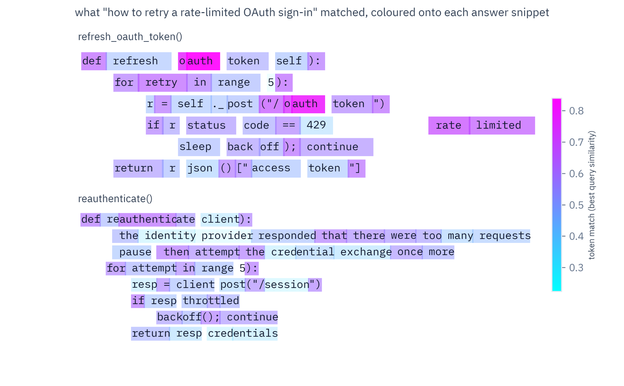
Query: How to retry a rate-limited OAuth sign-in?
maxsim://oauth-retry · token-match inspector
live similarity
Near exact-token match
Survives verbatim:rate limited OAuth
Soft / semantic match
authenticate ↔ OAuth retry ↔ attempt
Scoring happens token by token: we never have to choose between the two behaviors.
This is the late-interaction promise in one example. The query asks about retrying a rate-limited OAuth sign-in. The left console is deliberately translucent because the underlying plot has a transparent canvas: this keeps the token-level evidence legible without turning the visualization into a pasted white screenshot.
Some evidence should survive almost verbatim: "rate limited," "OAuth," perhaps a function or path. Other matches need to be soft: "authenticate" can support "OAuth," and "attempt" can support "retry."
Because scoring happens token by token, we don't have to choose between these behaviors or tune lexical-versus-dense fusion weights. We preserve strong exact-ish clues while still matching related language.
In the wider retrieval stack, late interaction usually replaces or strengthens first-stage dense retrieval; it does not make cross-encoders obsolete. A high-budget pipeline can still retrieve broadly, use late interaction to shorten the list, then reserve a cross-encoder for the final rerank. A pooled vector may also remain useful for questions about a document's global meaning, but its clearest practical advantage is still cost.
Punching above their weight class
MTEB(Code, v1) · source-deck snapshot · open benchmark
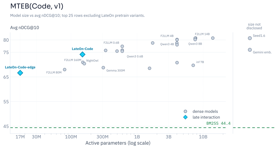
LateOn-Code 130M and LateOn-Code-edge 17M sit well above the BM25 baseline .They compare favorably with much larger dense models .
Public leaderboards shortlist; your repos decide .
The proof is in the pudding: model size on the horizontal axis, MTEB Code performance on the vertical. MTEB is the Massive Text Embedding Benchmark; the Code split evaluates code retrieval.
At LightOn we trained two code retrieval models: LateOn-Code, 130M params, and LateOn-Code-edge. Both late interaction. They sit well above the BM25 reference and compare favorably with much larger dense models.
This shouldn't tell you BM25 is dead, and public benchmarks are limited, but a late-interaction model can be very competitive for its size while retaining the local matching behavior code search needs.
There's more to agentic retrieval than accuracy
BrowseComp-Plus · cyan = late interaction · purple = dense models
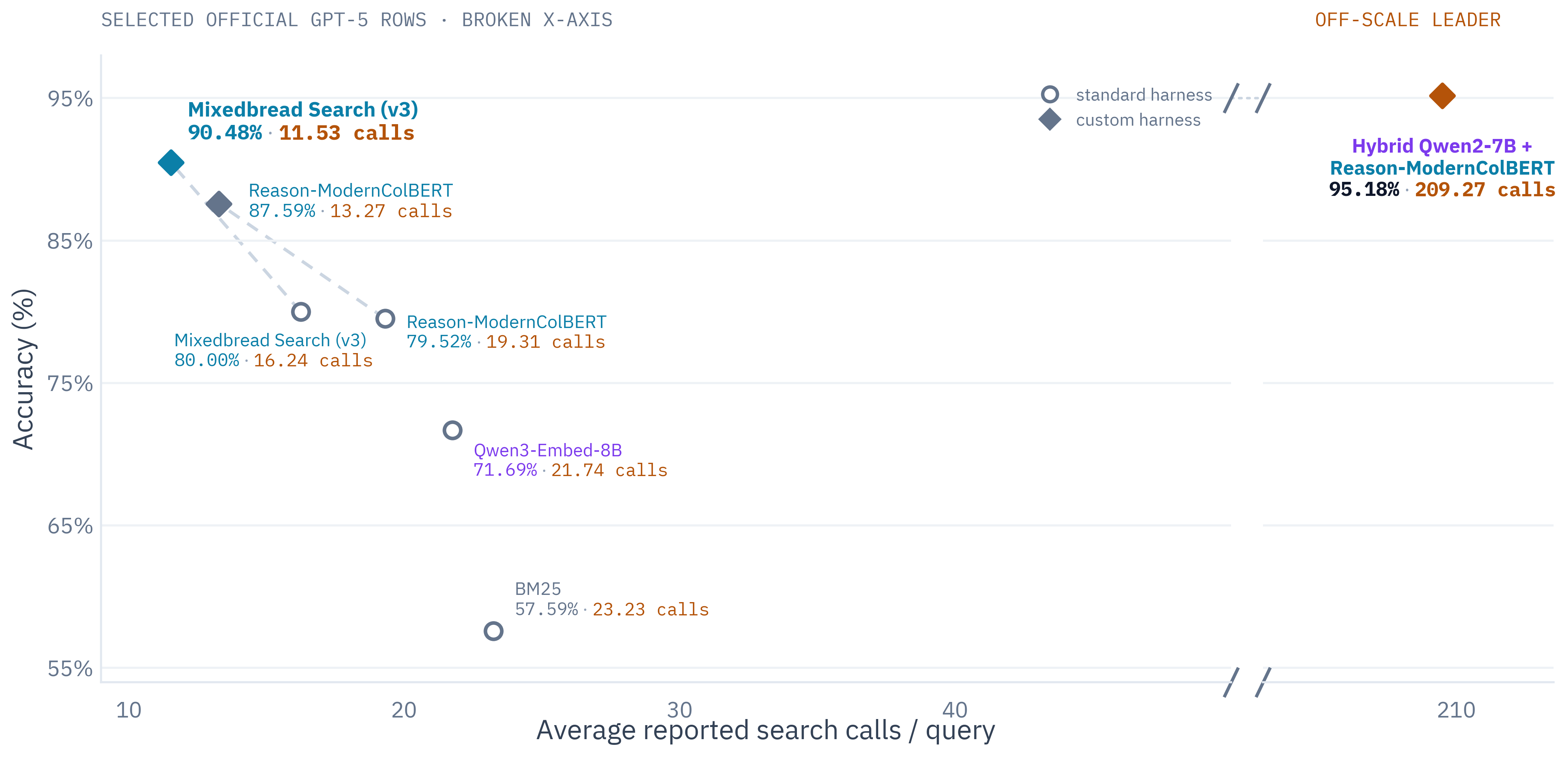
#1 hybrid system:95.18% accuracy at 209 search calls / query
#2 & #3 are late interaction : near-top accuracy at ~18× fewer calls , one of them at 150M params
Before moving away from code: why this matters in the real world. BrowseComp-Plus is a deep-research benchmark: 830 queries, ~100k documents. It reports both answer accuracy and average search calls, and the leaderboard is telling.
The current official top entry, with GPT-5, uses a hybrid Qwen2-7B + Reason-ModernColBERT retriever: 95.18% accuracy, but an average of 209 search calls per query. Imagine the cost.
#2, Mixedbread Search v3 (late interaction, closed-source), reaches slightly lower accuracy with about 18x fewer calls. #3, LightOn's Reason-ModernColBERT, is a couple of points behind at only 150M params, trained a year before the benchmark existed.
Takeaways: search-call count is becoming a first-class citizen, and late interaction achieves very competitive results while limiting it.
Search quality is an agent cost lever
Traditional IR
Optimizes for NDCG, MRR, Recall & Precision
→
Agentic IR
More recall oriented, optimizes for fewer search calls
The counterintuitive point: adding a dedicated retrieval model can make the full agent cheaper.
The bet: as CPU-friendly inference and local indexing mature, and late interaction models stay competitive while small, the gap narrows for tools such as ColGrep .
BrowseComp-Plus isn't a code benchmark, but its lessons apply directly to agentic code search.
FastContext reported that reading and searching make up more than half of tool-use turns and almost half of the main agent's tokens. The qualitative point is useful: traditional IR focuses on ranking metrics; an agentic system also cares about how many searches and reads are needed before useful work can begin.
It can feel counterintuitive that ADDING a dedicated retrieval model makes things cheaper, but if it reduces exploration, repeated calls, and context pollution, the full agent becomes cheaper and faster even though the retrieval step is more sophisticated.
02 FIELD CASE
Multimodal retrieval
Code makes exact-ish matches obvious. Visual documents make the compression problem obvious.
Now that we've seen the strengths of late interaction for code retrieval, let's move to the second field case. Code makes exact symbols obvious, so dense models suffer from diluting strong signals into a single vector. Visual documents make the compression problem obvious.
But before going multimodal multi-vector: why multimodal retrieval at all?
A picture is worth a thousand words
Sometimes, the evidence you're looking for is a clean text (code!) snippet. Sometimes it's just not.
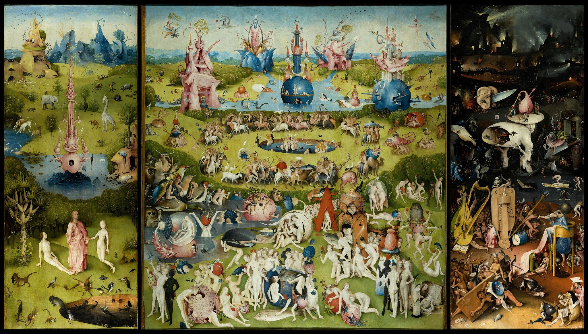
Consider this beautiful example I borrowed from Benjamin Clavié, and imagine my query was "a painting with a guy stuck in a mussel."
A traditional text retrieval pipeline could not deal with images unless it involved a captioning model. And when it comes to captioning: good luck with this one! It would have to guess in advance that this particular odd visual detail matters, or be very, very descriptive.
Direct visual retrieval keeps image regions available for matching instead of forcing the page through a text bottleneck first.
A picture is worth a thousand words
Sometimes, the evidence you're looking for is a clean text (code!) snippet. Sometimes it's just not.
ViDoRe v3 · Loison et al., 2026
Query
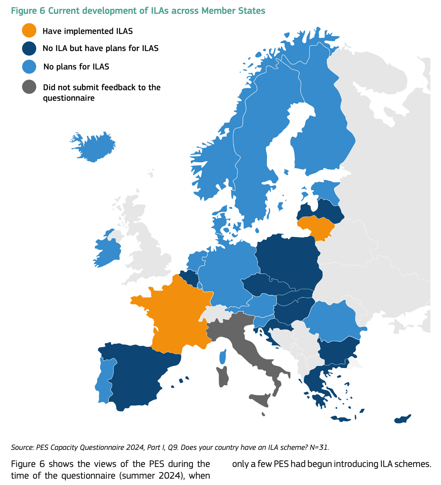
"Is there uniform interest across all EU regions in adopting Individual Learning Accounts?"
OCR + Chunking
Would only get the caption (if we're lucky).
You might say: cool, but I'm not trying to retrieve paintings! Fair, but a lot of enterprise documents contain visually-encoded information.
This query asks whether interest is uniform across EU regions. OCR might recover the caption and a few labels, but a captioning model would need to be specifically trained or prompted to transcribe this map, because the answer depends on the spatial pattern.
A generic caption may say "map of Europe" and miss the relevant distribution entirely. The retrieval lesson: preprocessing is not neutral. Whatever OCR or captioning fails to preserve is gone before ranking even starts.
Document Screenshot Embedding
Document lane
→
vision
→
one page vector
↘
ANN + the vectors
→
ranked pages retrieve first,
Query lane
"total revenuein Q3 "
→
text
→
one query vector
↗
familiar ANN pipeline
one page vector compresses every region, table & text zone
Technically, single-vector also works for images: one page image becomes one embedding, we train models to bring queries and matching pages together, and we can use a familiar ANN index. We can even rerank candidates with a vision model.
But notice we have recreated the dense retrieval bottleneck at the page level. The page may contain paragraphs, charts, labels, tables and footnotes, and we ask one vector to summarize all of it. A visually rich page is already a kind of long context: a lot of potentially useful information compressed into one representation.
From tokens to patches
Late interaction but for a page: split the image into a grid of patches , and keep one vector per patch.
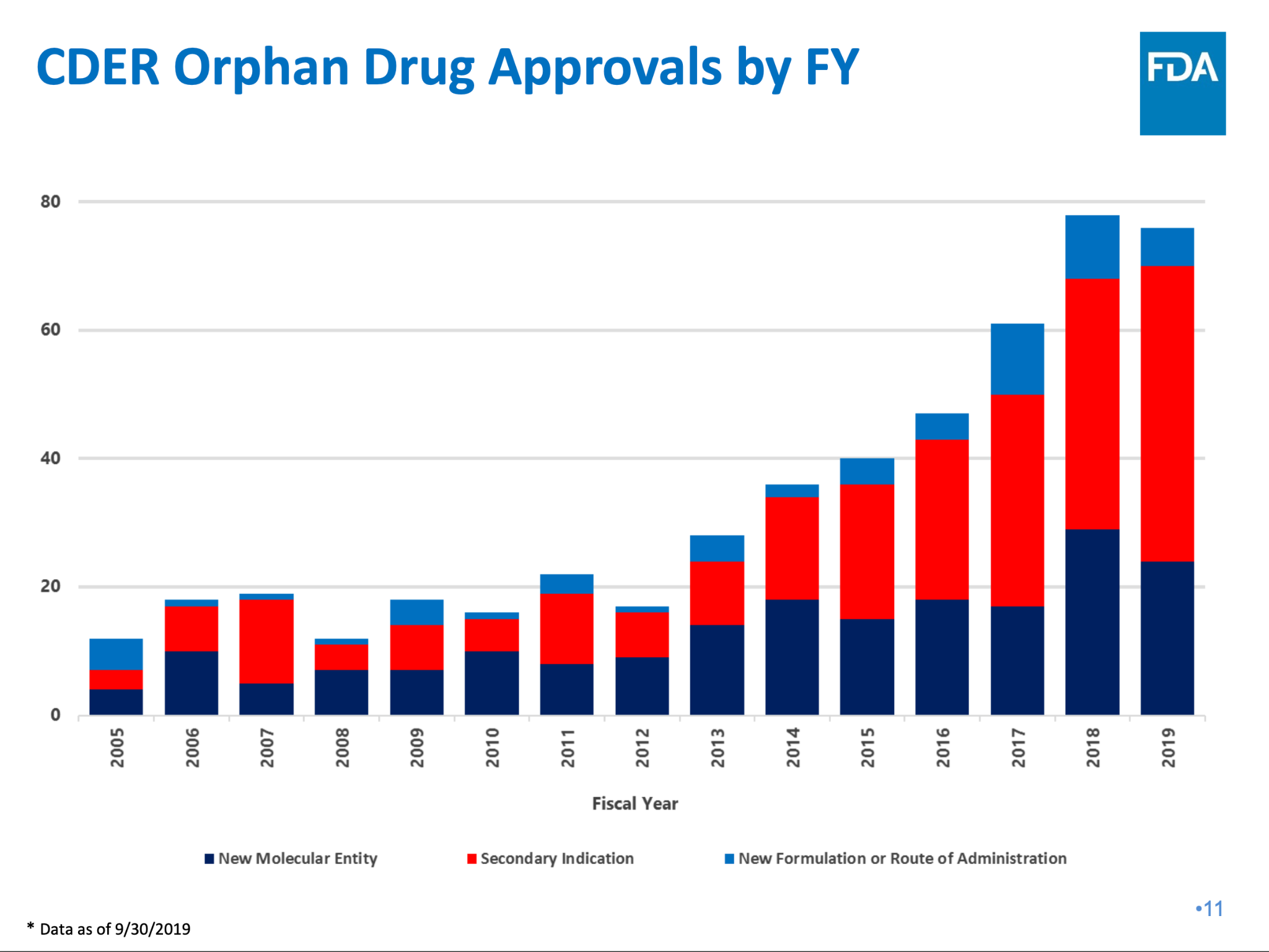
CDER Orphan Drug Approvals by FY FDA
New Molecular Entity Secondary Indication New Formulation
Page image + patch grid
encode
one page = N patch vectors
Patch-level evidence preserves local visual information, matched by MaxSim .
No single-vector bottleneck: the dates are not in the same patches as the caption, etc.
ColPali: Efficient Document Retrieval with Vision Language Models · Faysse et al., 2024
ColPali applies late interaction to a page image. For text we preserve multiple token vectors along a sequence; for a page we preserve multiple patch vectors across a two-dimensional layout. The geometry differs, but the retrieval idea is the same: keep local regions independently addressable.
We train the model to bring together query token-vectors and patch-vectors, and MaxSim lets each query token find the patch that best supports it. This removes the single-page-vector bottleneck: date labels, chart title, and relevant bars no longer compete for space inside one pooled representation.
Query-to-patch matches are visualizable!
Similarly to text highlighting: when a page is a match, you can see which regions of the page match which token from the query.
Query
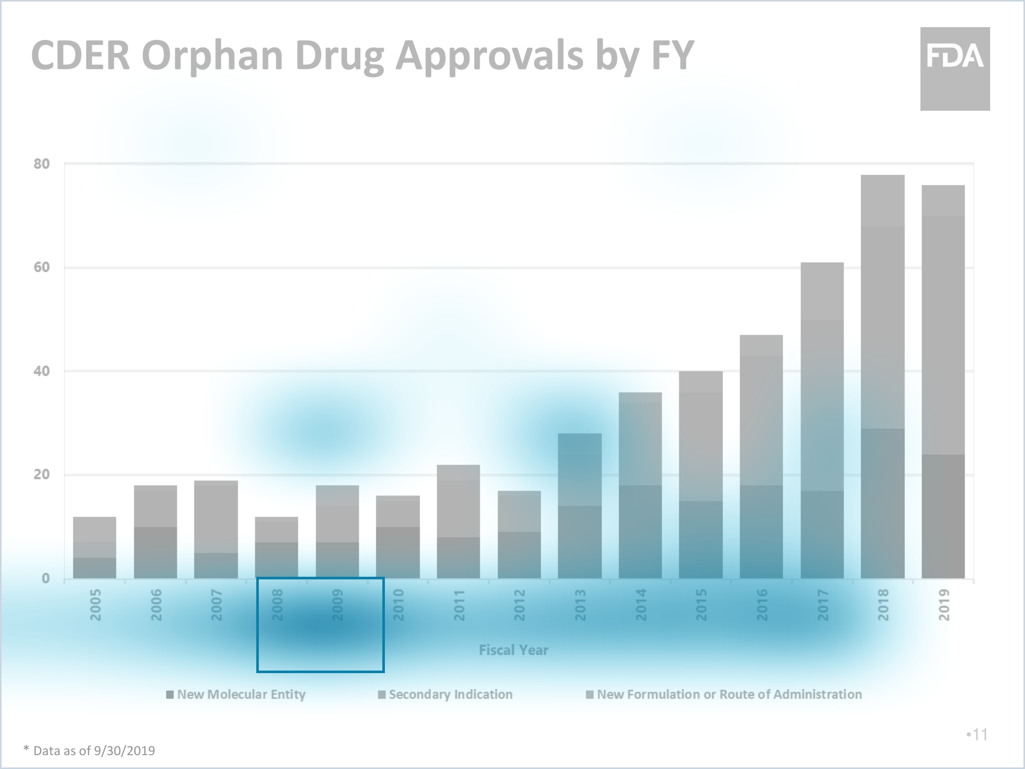
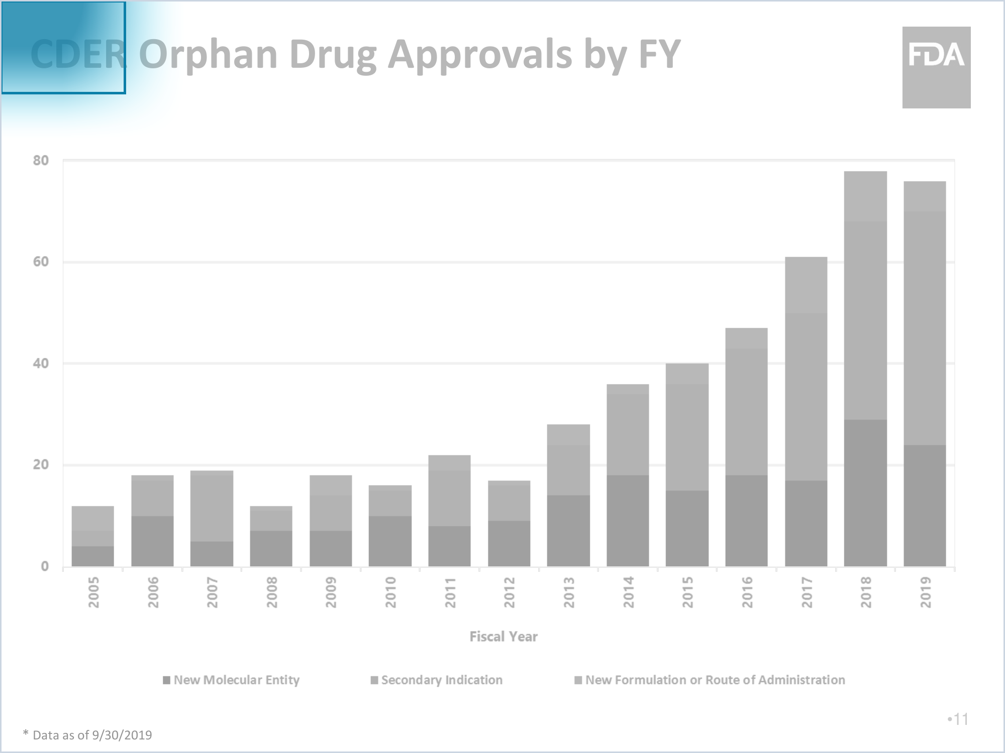
"Is there a rise in CDER NME submissions from 2007 to 2008 ?"
Evidence we hope the retriever notices: the two years , the relevant bars , and the title / legend .
Another benefit: we can inspect where the score came from. Same as text highlighting, but for visual retrieval: which image patch matched which query token.
Back to our query about CDER NME submissions from 2007 to 2008. Before revealing matches, identify the evidence we'd want the retriever to notice: the two years, the relevant part of the chart, and the legend that says which colors in the bars we should focus on. The next slides show those query-to-patch matches one token at a time.
If highlighting the page regions that support a result is a product requirement, this is a strong reason to evaluate multi-vector retrieval: the query-to-patch alignment comes from the scoring operation itself. A dense retriever would need a separate grounding or explanation model after retrieval.
Query-to-patch matches are visualizable!
Query: "Is there a rise in CDER NME submissions from 2007 to 2008 ?" · matching the token 2008
If we look at what matched best with 2008, we find the stronger associations around the x-axis, and the strongest match is indeed the 2008 patch!
Query-to-patch matches are visualizable!
Query: "Is there a rise in CDER NME submissions from 2007 to 2008?" · matching the token CDER
Finally, the CDER query token matched best with the title of the plot, which does contain CDER!
Punching above their weight class Dominating
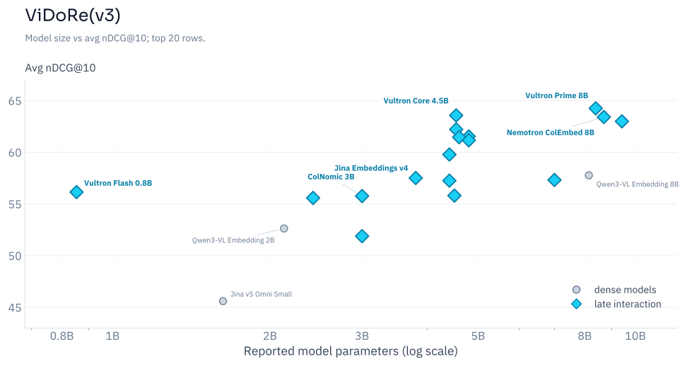
ViDoRe(v3) · source-deck snapshot · open benchmark
The top 20 is essentially all late interaction .
The few dense models that survive trail same-size late interaction by ~5 nDCG@10.
Visual retrieval suffers acutely in the single-vector compression bottleneck.
For vision retrieval, on ViDoRe v3 (Visual Document Retrieval benchmark), the story is not "late interaction punches above its weight" but "late interaction DOMINATES the leaderboard."
Not only are there few dense models for visual retrieval, the ones that exist noticeably lag behind late interaction models of similar size. A clear signal that visual retrieval absolutely suffers inside the single-vector compression bottleneck.
INTERLUDE
Out-of-domain,
Before moving to production objections, a short interlude: one strength of late interaction we haven't discussed yet is GENERALIZATION, and its strength on long context. We briefly touched on generalization when I said that in code search each repo has its own tiny vocabulary; let's dig a bit more.
"2008" still finds the right region
Query: "Is there a rise in CDER(?) NME(?) submissions from 2007 to 2008 ?"
Even if CDER and NME are poorly represented, another query token can still contribute a strong patch match .
A dense retriever summarizes the whole query in one vector: unfamiliar terms distort the summary , and the useful clues have no independent way to contribute.
Back to "Is there a rise in CDER NME submissions from 2007 to 2008?" Imagine our models have no idea what CDER or NME mean.
A dense retriever needs one vector that summarizes the whole query. If those unfamiliar terms distort that summary, even the useful clues such as 2008 have no independent way to contribute to the score.
With late interaction, even if the matches for CDER and NME are not meaningful, a token like 2008 will still be represented well enough to find its own best-matching patch and contribute useful evidence.
The document grows around the answer
The relevant span in a long document retains its local representation .
query token 2008
+100 passages local evidence intact
same local
Single vector As context grows, the answer becomes a smaller fraction of the global summary.
Late interaction The 2008 token keeps its own local vector, so the query can still reach it directly.
Now turn the same intuition around: from unfamiliar query terms to a growing document. A 2008 query token needs to match a "…rose in 2008" span. Imagine that passage gets progressively diluted into longer and longer context. I draw it as text, but the same picture applies to a visual page: add tables, figures and regions around the relevant patch.
A dense retriever must compress that increasingly large mixture into one vector: as more unrelated material is added, the relevant sentence becomes a smaller part of the global summary. Late interaction does not require one global meaning: the relevant span retains its own local representation, so 2008 can still find it, even buried in much more context.
No guarantee the document wins every time; longer documents add distractors. But it is an architectural reason for graceful degradation.
Late interaction is not magically independent of chunking: the encoder still has a finite context window, so very long inputs must be split. It is usually less brittle about the exact boundary, though, because a useful local token span does not have to dominate the pooled summary of its entire chunk.
Late interaction holds up under two shifts
Held-out languages stress the query; MLDR also stresses the document with long context.
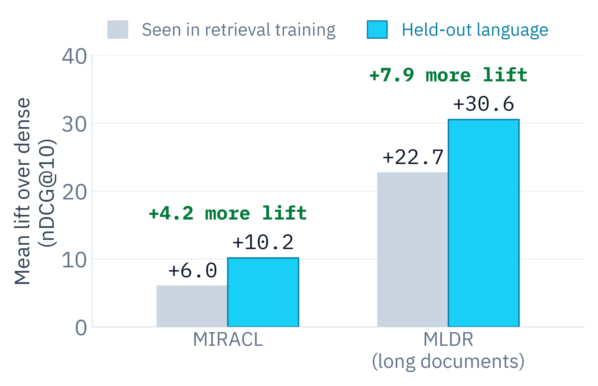
We trained two models: same backbone, same data recipe . One dense, one late interaction.
Evaluated on MIRACL (multilingual) and MLDR (multilingual + long documents).
On target languages, late interaction is already stronger .
On unseen languages, it generalizes better ; on MLDR the absolute gap is bigger.
LightOn multilingual DenseOn vs LateOn · lift over dense, nDCG@10
DenseOn with the LateOn: Fully Open Dense and Late-Interaction Models for Multilingual, Long-Context, and Code Search · Sourty et al., 2026
Now empirically. Something we discovered recently at LightOn that I find insanely interesting: we trained DenseOn and LateOn, then multilingual versions, with the same backbone and data recipe covering nine languages. We evaluated on MIRACL, a multilingual retrieval benchmark, and MLDR, multilingual and long-context.
On target languages, late interaction is already stronger; on unseen languages, the advantage grows significantly. What's crazy: the late interaction model stays competitive even on languages that don't share scripts with the training set. MLDR is particularly interesting because it contains long documents: the gap between dense and late interaction is much bigger.
These abilities depend on the backbone, mmBERT, having seen roughly 1,800 languages in pre-training. We did not teach the retriever Korean, but the encoder was not seeing Korean from scratch; late interaction lets those pretrained local token representations remain separately useful. This is not evidence that the method would understand a made-up language. It is evidence that retrieval training can transfer further when it does not have to compress every clue into one global vector. Does this only happen with text?
The same pattern survives a new benchmark
ViDoRe v3 arrived after release: an unseen benchmark for both models.
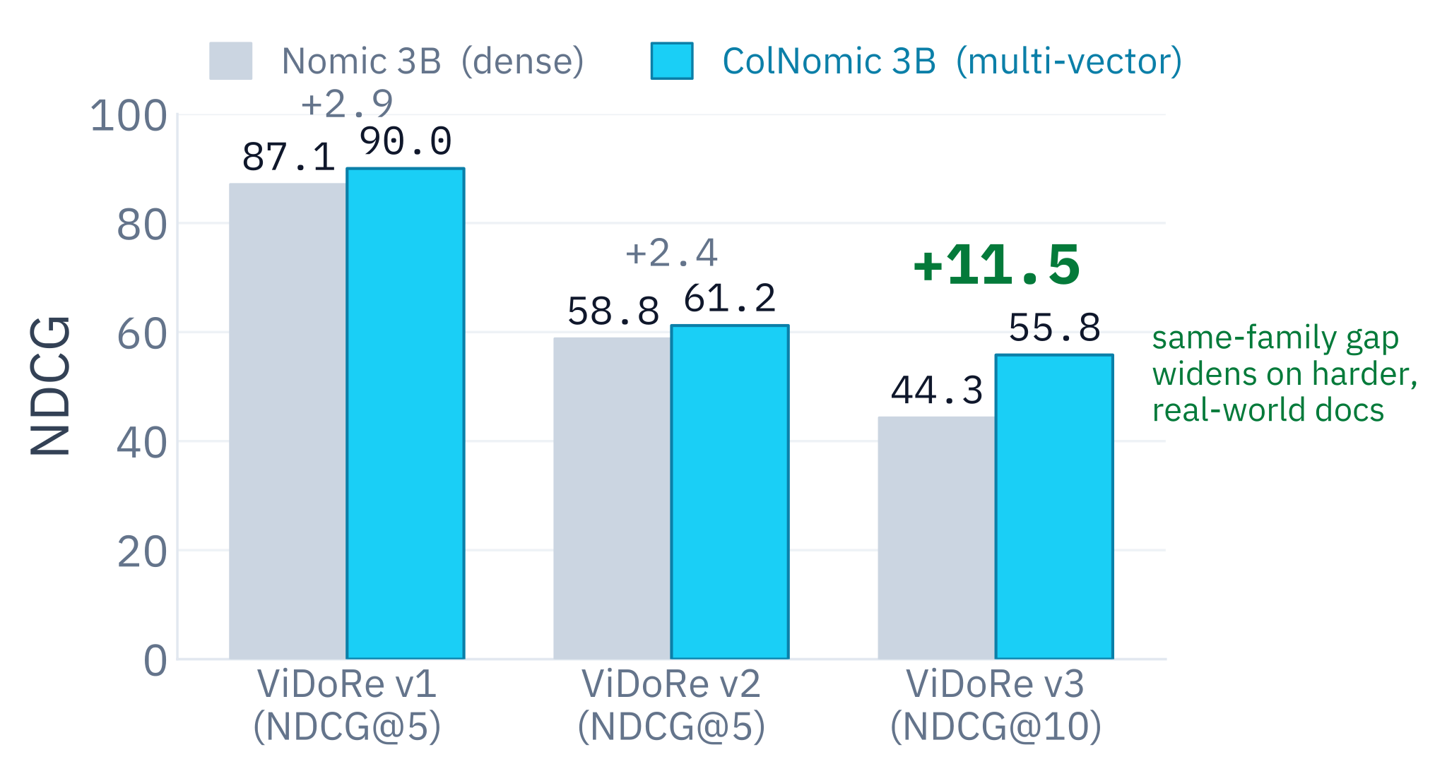
Nomic trained a dense and a late interaction multimodal 3B: same backbone, same data recipe .
At release, ViDoRe v1 and v2 existed; on those, late interaction was already stronger (+2.9, +2.4).
On v3 , unseen by both models, the gap widened to +11.5 .
Nomic model cards (v1, v2 · NDCG@5) · ViDoRe v3 leaderboard (NDCG@10)
We see a very similar pattern in visual retrieval. Nomic released a dense and a multi-vector model with the same backbone and data recipe, before ViDoRe v3 existed. On v1 and v2, the multi-vector model was better, but modestly: roughly two or three points.
ViDoRe v3 is a useful natural stress test: a new benchmark with harder, more realistic documents and a different distribution. On that unseen benchmark, the gap grows to 11.5 points.
This is by far the most controlled comparison we have, but we also saw other dense retrievers that were decent on v1 and v2 get much worse on v3.
ONE GLOBAL REPRESENTATION CAN BE BRITTLE · LATE INTERACTION SAVES THE DAY
But why isn't
We have now seen the same pattern across unfamiliar languages, long documents and visual pages. Different retrieval tasks, same pressure: the global representation becomes less reliable, while useful local evidence may still survive.
So why isn't late interaction the default? Because preserving all those local pieces of evidence is not free. We now have many vectors to store, retrieve and score.
Why late interaction isn't the default
02
Retrieval is too slow.
03
The model ecosystem is too narrow.
In the big 2026
Which objections are still fundamental, and which are becoming engineering problems ?
The traditional objections are straightforward: the index is too large, retrieval is too slow, and the model ecosystem is too narrow. We'll examine each rather than hand-wave them away. This deck follows the unusually active 2026 research wave, then asks the useful 2027 deployment question: which costs are fundamental to keeping more evidence, and which have become manageable engineering trade-offs because compression, indexing, and tooling improved?
A lot of the work in this section is frontier work, but the point is that each objection now has several concrete lines of attack.
01 OBJECTION
The index is too big
We start with storage because it is the easiest cost to quantify, and because the naive numbers are deliberately alarming.
The naive baseline
Naive storage math:index size = tokens/doc × docs × dims × bytes
MS MARCO: ~80 tokens × ~9M passages × 128 dims × 4 B (fp32)
~369 GB
for one MS MARCO index.
Compared to single-vector, with 2,048 dims:73 GB
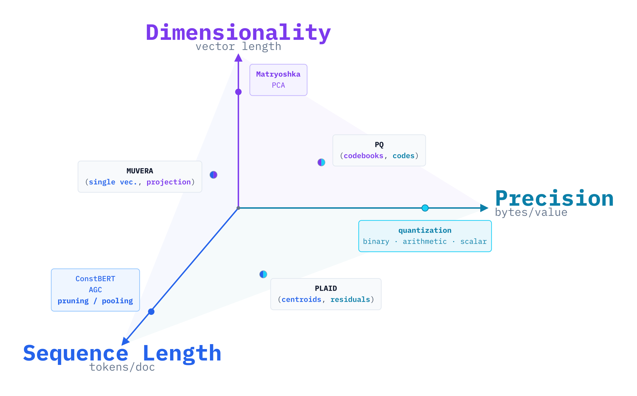
Three levers to pull → · Jha et al., 2026 (poster redraw)
The formula is simply vectors per document times dimensions times bytes times document count. With roughly 80 token vectors per MS MARCO passage, 128 dimensions, fp32, and 9 million passages, the naive estimate is about 369 gigabytes.
A single-vector index with a much wider 2,048-dimensional embedding is only about 73 gigabytes, because there is one vector per passage rather than 80. That comparison is the point: dimensionality alone does not determine storage; sequence length matters enormously, as does precision.
Rohan Jha made this excellent figure showing the levers we can pull to reduce index size. Let's dig in.
Centroid ID + tiny residual per token
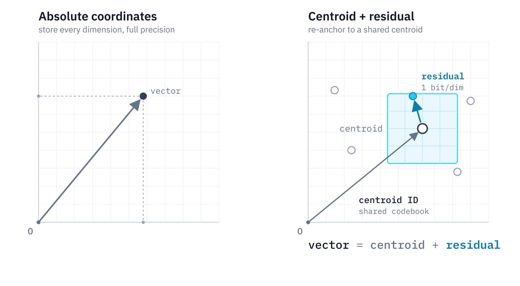
ColBERTv2 introduced residual compression as a key late-interaction storage technique: vector = shared centroid + low-bit residual .
K ~ 16 √(docs × dim) centroids, shared across the whole index
Strategy Bytes / token MS MARCO
Naive · fp32 512 B 369 GB 2-bit residual 36 B 25.9 GB 1-bit residual 20 B 14.4 GB
Preserve the multi-vector shape without preserving every float: now below the 73 GB single-vector baseline.
ColBERTv2: Effective and Efficient Retrieval via Lightweight Late Interaction · Santhanam et al., 2022
First lever: precision. ColBERTv2's residual compression: instead of storing every token vector in full precision, store a shared high-precision centroid table, then a centroid ID and a tiny low-bit residual per token. The centroid table is SHARED, so you pay once per centroid rather than once per token, and the paper finds the number of centroids scales as the square root of docs times dims: sublinear.
Back to the MS MARCO napkin math: at 128 dims the naive vector costs 512 bytes; a 2-bit residual plus ID is about 36 bytes per token; 1-bit is about 20. That takes the index from 369 GB to roughly 25.9 or 14.4. We preserve the multi-vector shape without preserving every float.
How far can precision go?
Precision can be asymmetric : the corpus is stored, cached, and re-scored over and over; the query is tiny and short-lived → keep the query sharp and push the document side much lower.
Configuration Storage / doc NDCG@10 Latency
fp32 q × fp32 d 393 KiB 90.26 14.20 ms int8 q × binary d 12.28 KiB 89.65 3.71 ms
The asymmetry
query · int8 8 bits / value binary 1 bit / value
32× smaller document vectors
−97% storage per document
−0.61 NDCG@10 · near lossless
Asymmetric quantization · Mixedbread, 2026
Recent work by Mixedbread pushes much further: precision does not have to be symmetric. The query is tiny and short-lived, while document vectors are stored and scored repeatedly. So keep the query relatively sharp and compress the document side much harder.
In their reported setup, int8 queries against binary document vectors reduced storage per document from 393 to about 12 KiB and latency from 14.2 to 3.71 ms, while NDCG@10 moved from 90.26 to 89.65. Which is to say, barely.
This is frontier work, but a striking and encouraging result.
How many vectors is multi-vector?
Single vector N = 1 vector
In between?pool or prune
Usual late interaction N = ntokens vectors
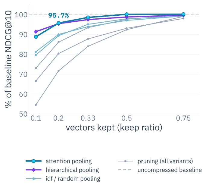
GTE-ModernColBERT-v1 · BEIR+CoIR · % of baseline nDCG@10
Pooling beats pruning.
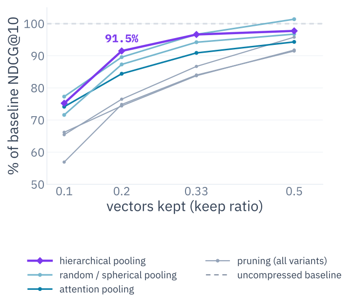
Hierarchical / attention pooling holds ~96% of baseline NDCG@10 at just 20% of the vectors .
Similar findings for visual retrieval (bonus slides).
A Brief Comparison of Training-Free Multi-Vector Sequence Compression Methods · Jha et al., 2026
Second lever: sequence length. If single vector means pooling every token into one, and multi-vector means one vector per token, can't we do something in the middle? Yes: two families. Pruning drops token vectors, randomly or by rule; pooling merges some together.
The training-free comparison by Rohan Jha and colleagues finds two things: first, the results favor pooling. Intuition: pruning deletes evidence; pooling combines redundant evidence while keeping every region represented.
Second, and impressive: hierarchical or attention pooling keeps around 96 percent of baseline quality with only 20 percent of the vectors. That translates directly into index size.
Documents do not need to end with a constant number of vectors: an index can store a variable-length token matrix per document. The late-interaction compression work cited here reduces that count by merging or assigning token vectors with hierarchical clustering, spherical k-means, sequential grouping, or attention-based pooling.
Remember, here we reduce how many vectors represent the sequence; Matryoshka-style truncation later reduces the width of every vector.
How far can sequence length go?
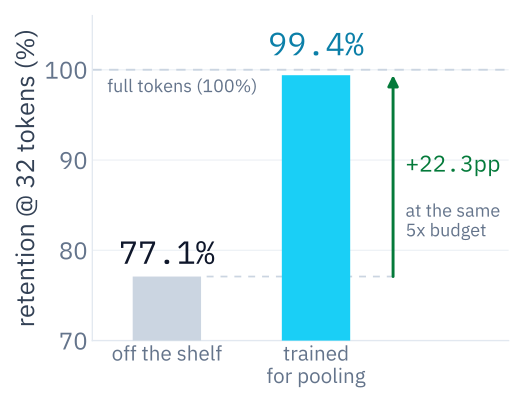
Merging similar token vectors already cuts the index essentially for free. Train the model for pooling , and 5× compression becomes near-lossless.
LateOn · 32 tokens/doc = 5× compression · % of full-token nDCG@10
Nothing changes at query time
one fine-tune · the model simply learns to be easy to compressone index build · pick the compression ratio at inference timeadaptive budgets · tokens flow from redundant docs to dense ones, free
99.4% retention at 5× compression
Same pattern in vision: after merge-aware fine-tuning, Light-ColQwen2 retains 94.6% at 49× patch compression (2% index size).
Regularizing ColBERT models for pooling · Chaffin, 2026 · pooling-aware training proposed independently by Stefan Josef in Learn to Pool
How far can we go on this axis? Hierarchical pooling is already a great default without special training. The 2026 update: the ceiling is not fixed. If the model is fine-tuned to be compressible, the same five-times compression becomes near-lossless: 99.4% retention, with full-token quality unchanged.
The same qualitative pattern appears in vision: a merge-aware fine-tuned Light-ColQwen2 retains 94.6% of full-model NDCG@5 at factor 49.
Takeaway: training turns pooling from "nice, small quality tax for a smaller index" into a near-lossless process across modalities.
Matryoshka for late interaction
Shrink every token vector: train the widths jointly, pick one at index time . Storage and MaxSim compute are both linear in width.
Jina-ColBERT-v2
six widths trained jointly (MRL), chosen at index time · BEIR ablation, fp16
128 d · 256 B/token
baseline
96 d · 192 B/token
close to baseline
64 d · 128 B/token
−1.59% nDCG@10 · half the index
MM-Matryoshka · vision
The same width elasticity for vision, with encoder depth elastic too.
The crucial rule: use a width the model was trained for . Arbitrary truncation is not the same thing.
Jina-ColBERT-v2 · MM-Matryoshka
Third lever: vector width. Matryoshka training makes one model useful at several dimensions, so you can choose the width to serve. It pays twice: storage is linear in width, and so is the cost of each MaxSim dot product.
For text, Jina-ColBERT-v2 was as far as I know the first to explicitly train a late interaction model with Matryoshka representation learning: the 64-dimensional head halves the index for a relatively small reported quality loss.
On the vision side, MM-Matryoshka makes both width and encoder depth elastic. The crucial rule: use a width the model was trained for; arbitrary truncation is not the same thing.
Stack the levers, evaluate the stack
Each axis is cheap on its own, measured on its own .
Precision
2-bit residuals
nbits=2
quality-neutral, measured alone
×
Sequence length
token pooling ×2
pool_factor=2
near-free, measured alone
×
Width
Matryoshka 64 d
dim=64
small cost, measured alone
The storage savings multiply! But the quality costs may compound → be aware of it, keep the knobs explicit and evaluate on your own queries .
The previous slides pulled the three axes one at a time; in production we can in theory stack them: low-bit residuals, fewer pooled vectors, and a narrower trained head.
The storage savings multiply, which is why multi-vector indexes can shrink by an order of magnitude or more. The quality costs may also interact, though, and each number was measured mostly in isolation. Keep the knobs explicit (nbits, pool_factor, dim) and evaluate the actual combination you plan to ship. The full stack on your data matters more than three reassuring ablations from separate experiments.
02 OBJECTION
Retrieval is too slow
Once we've handled index size, the next obvious objection: even if the index fits, MaxSim looks expensive. Next we separate the simple mathematical definition from the way real systems actually retrieve.
Naive MaxSim is doomed
query tokens
~32
every query token needs its best document-token match
×
tokens / passage
~80
all token pairs are scored inside one passage
×
MS MARCO passages
~9M
repeat the all-to-all comparison for the whole corpus
=
per query
~23B
dot products at dimension 128
Exact MaxSim is the target score , not the first-stage search plan.
If we consider MaxSim naively, comparing every query token with every token in every document, the arithmetic explodes. For MS MARCO: roughly 32 query tokens times 80 document tokens times 9 million passages gives around 23 billion dot products, each at dimension 128.
Obviously not a viable first-stage search. The important point: no serious system implements exact MaxSim over the whole corpus. MaxSim is the target score; efficient retrieval is about reaching a good candidate set without paying that target cost everywhere.
Every fast system is a funnel
Two things change on the way down: the set shrinks, the price per document rises .
The set · shrinks ↓
All documents · ~9M
↓
Candidates · ~100k
↓
Shortlist · ~1k
↓
top-10
The scorer · cost per doc rises ↓
1
Candidate generation
using a cheap scoring method · cheap
2
Approximate MaxSim · prune
refine further if need be · moderate
3
Exact MaxSim
only on a much smaller number of survivors · expensive
The whole speed / quality trade-off is one question: how many documents reach exact MaxSim?
The common pattern to make retrieval fast is a funnel: start broad and cheap, then spend expensive scoring only on a smaller set. Begin with all documents and a cheap candidate-generation score; prune aggressively; use a more faithful approximate score on fewer candidates; reserve exact MaxSim for a small shortlist. As the set shrinks, we can afford a more expensive score per document.
The central speed-quality knob is not mysterious: how many documents survive long enough to receive exact scoring? The counts here are illustrative, but the funnel pattern is common across systems.
PLAID
Use compression for candidate generation: coarse first, exact only for survivors . Offline: select centroids, assign each token to its nearest one, store centroid ID + 1-2 bit/dim residual.
1 Score centroids
query tokens centroid codebook
Score every query token against the shared codebook.
2 Gather candidates
d4 · d9 · d2
d2 · d7
d9 · d1 · d5
Pull documents from each token's top-nprobe centroid lists.
3 Approximate MaxSim
Score documents as bags of centroids, nothing decompressed yet.
4 Prune hard
d4 keep
d9 keep
d2 drop
d7 drop
Keep a shortlist of ndocs candidates.
5 Full-score survivors
Decompress residuals, rebuild real vectors, run full MaxSim.
exact scores · few docs
Residual work is reserved for the survivors.
up to 7× on GPU · 45× on CPU
lower latency than vanilla ColBERTv2, same quality
PLAID: An Efficient Engine for Late Interaction Retrieval · Santhanam et al., 2022
Starting with PLAID, which cleverly reuses compression for candidate generation. Remember ColBERTv2: token vectors decomposed into a centroid codebook plus low-precision residuals.
At query time, centroid-level interactions cheaply identify promising documents (centroids are shared!); residuals and exact token vectors are consulted only for survivors. The centroid does two jobs: saving storage and narrowing the search.
Introduced in 2022, with up to seven times lower latency on GPU and 45 times on CPU versus vanilla ColBERTv2, at the same quality setting.
Conceptually, PLAID plays the role that an approximate-nearest-neighbor index plays for dense retrieval: it is the approximate first stage that makes the exact target score affordable. In most products this logic belongs in the retrieval engine rather than in application code.
From research idea to system
A compression trick becomes a candidate generator, a fast backend, then a production API!
2021
ColBERTv2
Compressed late-interaction vectors
6-10× smaller index
via residual compression
2022
PLAID
Centroid-based candidate generation
up to 7× GPU · 45× CPU
vs vanilla ColBERTv2
2025
FastPlaid
High-performance backend
up to +554% QPS
vs PLAID · Rust, GPU
2025
NextPlaid
Production API + CRUD support
add / delete / filter
REST API · CPU-first
Two knobs make the trade-off visible: n_ivf_probe widens candidate generation · n_full_scores spends more exact MaxSim.
Since then, the algorithm is becoming infrastructure. ColBERTv2 compresses the index. PLAID turns the compression structure into candidate generation. FastPlaid focuses on a high-performance Rust and GPU backend. NextPlaid adds production concerns: REST APIs, filtering, CRUD.
Across the lineage, two knobs make the trade-off visible: n_ivf_probe widens candidate generation, while n_full_scores spends more exact MaxSim scoring. Turning either up tends to improve recall and cost more time.
Another route: MUVERA
Make candidate generation look like dense ANN , then keep late interaction for the rerank.
Doc token vectors
a set of vectors per document
Fixed-dimensional encoding (FDE)
b1
b2
b3
b4
2 · aggregate per bucket
b1 b2 b3 b4
3 · concatenate once
query: sum · document: mean · one vector stands in for the whole set
Any dense ANN index
→ candidates
off-the-shelf MIPS or vector-DB machinery
Rerank with MaxSim
full late interaction, candidates onlyfinal ranking
original token store
+10% recall · −90% latency
FDE(Q) · FDE(D) ≈ Chamfer(Q, D) = Σq∈Q maxd∈D q · d
A single dot product approximates multi-vector similarity, with provable ε-guarantees.
MUVERA: Multi-Vector Retrieval via Fixed Dimensional Encodings · Jayaram et al., 2024
MUVERA takes a different route: we know how to make dense search efficient, so can we make late interaction into dense search?
The paper shows you can convert a set of token vectors into a fixed-dimensional encoding that approximates multi-vector similarity, searchable with ordinary dense ANN infrastructure. That encoding generates candidates, while the original late-interaction vectors are kept for final reranking. First stage looks like dense retrieval; last stage still MaxSim.
Reported aggregate: large latency reduction and better recall than PLAID in that setup. The catch, which we'll return to: the token-vector geometry must cooperate with the random projections.
Sparse route: back to the inverted index
Three 2026 efforts plug token vectors into the classic posting-list workhorse!
Token vectors
from your late
→
Random anchors · SMVE
Plain-text SAE · Latent terms
Retrieval SAE · SSR
→
Inverted index
"refresh" → doc 3 · doc 8 · doc 21"oauth" → doc 1 · doc 8"429" → doc 8 · doc 13
→
Candidates
cheap, from mature
→
keep the 8 strongest per token
token vectors
random anchors (2048)
Post hoc: random anchors turn the token set into one sparse sketch.
doc = many token vectors
the SAE runs on every one
encoder
we keep this: the sparse middle
32,768 latents · 16 fire per token
decoder
reconstruction ≈ input
only the training signal;
A plain-text sparse autoencoder exposes a vocabulary for BM25-style indexing.
query tokens
doc tokens
neurons
f_812
f_047
f_310
score(q, d)
fires on one side only
→ adds 0
pairs meet only on shared neurons
A retrieval-trained SAE keeps sparse MaxSim in neuron space.
The last route for building the funnel: the SPARSE family, mapping token vectors into sparse keys so we can reuse posting lists, the classic inverted-index workhorse. Reminder: an inverted index is organized by terms, each term pointing to the documents containing it.
Three recent approaches: SMVE uses random anchors and keeps strong projections. Latent Terms trains a sparse autoencoder to expose a vocabulary indexable with BM25-like machinery. SSR also learns a high-dimensional sparse representation for neuron-level indexing.
Details differ, but the funnel is the same: create candidates cheaply with mature sparse infrastructure, then recover the richer MaxSim-style score on a smaller set, or approximate it directly.
The sparse keys still start from contextualized token vectors, not raw tokenizer IDs. That is why "glasses" can activate territory related to "spectacles": the semantic context is baked in before sparsification. This is philosophically close to learned sparse retrievers such as SPLADE, and I expect the two families to converge. Of the three examples here, SSR trains the retriever for its sparse representation; Latent Terms trains a sparse autoencoder without changing the base retriever; SMVE is fully post hoc.
Late interaction now reaches tens of milliseconds
← faster slower →
Frontier overlap single digits → tens
Modern multi-vector tens of milliseconds
Older / heavier hundreds of milliseconds
What changed
Centroid pruning, sparse coding, optimized kernels and hierarchical indexes can now put late interaction in an interactive latency regime .
Do not make a fake leaderboard
Hardware, corpus size, recall target, candidate depth and batching all differ. Compare latency within a paper, not across papers.
Representative territories, not normalized measurements · each method name links to its paper or implementation
"Fast" needs context: which hardware, which corpus, which recall target, and which product loop? If an LLM takes seconds, spending tens of milliseconds on stronger retrieval can be an excellent trade. For autocomplete, the same latency may be too expensive.
The source deck collected exact numbers from several papers, but those figures were not normalized to the same setup. There is no trustworthy universal latency-versus-accuracy Pareto chart yet: providers benchmark different hardware, corpora, query loads and recall targets. This version deliberately shows broad territories instead of a fake cross-paper leaderboard. The defensible conclusion is narrower and still useful: optimized late-interaction systems have reached interactive regimes, including tens of milliseconds in published setups, and the correct comparison is always within one paper or one controlled evaluation.
For keeping up with the field, the TusKANNy research group maintains an excellent Awesome Multivector Retrieval index of papers, models, engines and datasets; the same group produced TACHIOM, one of the frontier systems shown here.
03 OBJECTION
The ecosystem is too narrow
To finish up, the last objection you may have: there aren't that many multi-vector models available, it's a niche thing.
The model zoo is expanding
From "there are no models" to "which model fits my constraints?"
681 HF candidates · 19 curated releases
Multilingual text retrieval
2021 2022
2023 2024
2025 2026
The ecosystem objection has weakened substantially. A few years ago, late interaction often meant a small set of English text checkpoints and bespoke research code. Now there are models for multilingual retrieval, code, and visual documents, at a wider range of sizes.
That doesn't mean every domain is covered; it means the practical question has changed from "does a model exist?" to "which model fits my language, modality, memory, latency, and update constraints?"
Familiar tools for late interaction
~/retrieval/awesome_lateinteraction.py
PyLate · Python
from sentence_transformers import SentenceTransformer, evaluation as st
from pylate import models, evaluation as pl
dense = SentenceTransformer ("lightonai/DenseOn" )
dense_evaluator = st.NanoBEIREvaluator (dataset_names=["SciFact" ])
dense_results = dense_evaluator (dense)
late = models.ColBERT ("lightonai/LateOn" )
late_evaluator = pl.NanoBEIREvaluator (dataset_names=["SciFact" ])
late_results = late_evaluator (late)
Sentence-Transformers made dense retrievers' training & evaluation easy.PyLate plays that role for late interaction!
familiar model interface
training & evaluation
indexing tools
PyLate: Flexible Training and Retrieval for Late Interaction Models · Chaffin & Sourty, 2025
Tooling is what turns an architecture into something people actually adopt. Sentence Transformers made dense retrieval approachable with a simple model, training and evaluation workflow.
At LightOn we've worked on PyLate, which aims to provide that same experience for late interaction, sticking as close as possible to the sentence-transformers flow. As a user you shouldn't need to rebuild the research stack just to test the retrieval paradigm.
Fine-tuning a pretrained late-interaction model on domain data is common. Catastrophic forgetting remains a general fine-tuning risk, but in practice these models are not unusually difficult to adapt when the learning rate, data mix and evaluation remain sane. Keep a broad held-out set next to the domain eval so gains on the target corpus do not hide a generalization collapse.
Shortlist on MTEB, then verify on your data
Public numbers shortlist; your queries decide . The good news: late interaction models generalize better!
BEIRnDCG@10 · original rank
Decontaminated BEIRnDCG@10 · new rank
LateOn 57.22 pplx-embed-v1-0.6b 56.70 DenseOn 56.20 pplx-embed-v1-late-0.6b 56.11 jina-v5-text-nano 56.08 ColBERT-Zero 55.82 arctic-embed-l-v2 55.55 Qwen3-Embedding-0.6B 55.33 GTE-ModernBERT 55.19 harrier-oss-v1-0.6b 55.04 GTE-ModernColBERT 54.22 colbert-small 53.79 modernbert-embed-base 52.89
#1 61.36 #2 59.95 #3 59.84 #4 59.67 #5 59.29 #6 58.83 #7 58.81 #8 58.05 #9 57.98 #10 57.92 #11 56.96 #12 56.63 #13 55.61
BEIR nDCG@10 vs decontaminated BEIR · rank movement, not score movement
We decontaminated BEIR : removed samples found in large retrieval training sets.
Ranks move, sometimes a lot , though the models did not change.
Late interaction models consistently move up when contamination is removed.
Since we're talking about choosing a model: my closing words are to use public leaderboards to narrow to a few candidates, then run your own evals to make actual decisions. Public leaderboards do not say which model was benchmaxxed or which training set was contaminated.
The good news: late interaction models do surprisingly well out of domain. This figure shows recent work where we decontaminated BEIR, removing samples found in large retrieval training datasets: late interaction models consistently went up in rank when that was done, versus dense models.
What does "multi-vector support" actually mean?
Questions to ask your vendor
Is MaxSim first-stage retrieval , or second-stage reranking only?
If first-stage: what is approximate , and when is exact scoring recovered?
How do updates interact with compression?
How was the published quality / latency point measured ?
Most Vector DB vendors nowadays have late interaction support ! But the phrase hides very different implementations.
The message of the last three sections
In 2026 multi-vector search is production-usable : the compression and speed methods you just saw are real, and the main vendors already ship many of them. What stays yours is the trade-off: quality vs storage vs latency vs freshness . Now you know what to look for.
I expect most of you don't want to build your own vector DB or reimplement PLAID. My goal with this section is to make provider conversations sharper.
Some systems store real multi-vector fields and compute MaxSim-style scores; others use late interaction only for second-stage reranking. Ask whether MaxSim is first-stage or rerank-only. If first-stage, what is approximate, and when is exact scoring recovered? Ask how updates interact with compression and how the published quality/latency point was measured.
Implementations genuinely vary: Weaviate has pushed MUVERA; other engines expose native multi-vector fields or PLAID-like flows; several vendors recommend late interaction only as a reranker because their first-stage index does not optimize MaxSim. That is an infrastructure constraint, not proof that rerank-only is the only valid architecture.
The methods exist: compression makes the index affordable, funnels and projections make it fast, and the ecosystem is adapting. My prediction from the transcript is that sparse candidate generation will become mainstream, model trainers will increasingly optimize checkpoints for the target index, just as Matryoshka training became normal for dense retrieval, and vector databases will converge once one efficiency/quality frontier proves durable. What I hope you take away is a feel for the trade-offs and the questions that expose them.
What we covered
01
The bottleneck
One vector is the wrong shape for many relevance clues.
02
MaxSim & late interaction
Keep token / patch vectors; match locally at query time.
03
Two field cases
Code and visual documents: granularity and compression.
04
Production
Storage, speed, models & tooling.
Across text, code, languages and visual documents, late interaction repeatedly beats single-vector dense retrieval . The question now is how to deploy that quality edge efficiently.
The guide compresses into four ideas. First, one vector can be the wrong shape when a document contains many independent relevance clues, which is very often. Second, late interaction keeps token or patch vectors and uses MaxSim to match locally. Third, code and visual documents show why granularity and compression matter. Finally, the production costs are real, but precision reduction, vector pooling, narrower trained heads, retrieval funnels, and better tooling make them much more manageable than they used to be.
Field guide / complete
Thank you. Keep the evidence local.
Take one retrieval problem you already own, run the comparison, and let the numbers decide.
Amélie Chatelain, PhD LightOn · @AmelieTabatta
The closing invitation is deliberately direct: the tooling, model checkpoints, benchmarks, and production-oriented implementations now exist, so go test late interaction on your own retrieval problem. The links on this slide point to the people advancing the field and to TusKANNy's maintained Awesome Multivector Retrieval collection of papers, models, libraries, and systems.
A picture is worth a thousand words
Sometimes, the evidence you're looking for is a clean text (code!) snippet. Sometimes it's just not.
Query
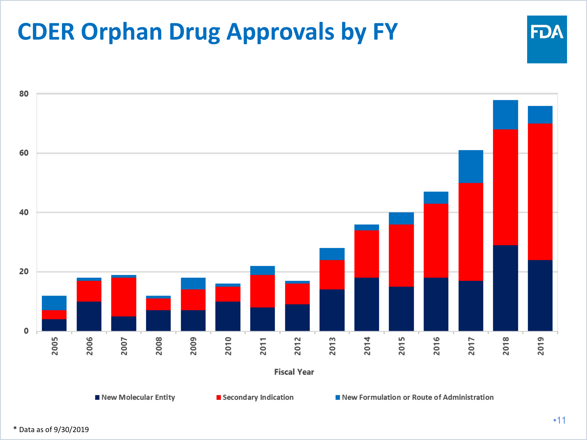
"Is there a rise in CDER NME submissions from 2007 to 2008?"
OCR + Chunking
Would require approximating each value in each bar…
Last example, showing the power of working in the vision space: this question asks about a change from 2007 to 2008.
For a text retrieval pipeline, we would need to estimate each bar's value to convert the chart into structured data. Possible in theory, expensive and brittle in practice. In comparison, it is attractive to retrieve from the page image itself and compare relatively: the red box in 2007 versus the red box in 2008.
A picture is worth a thousand words
Sometimes, the evidence you're looking for is a clean text (code!) snippet. Sometimes it's just not.
Query
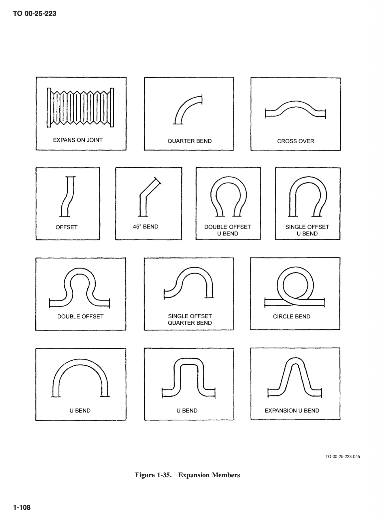
"number of hose installation diagrams · pressure systems manual"
OCR + Chunking
Without layout detection, would be much harder.
Another example: the query is about the number of hose installation diagrams in a manual. The relevant signal is partly textual, partly visual, and partly structural.
Without layout detection, OCR gives a bag of fragments but may not tell us which fragments belong to separate diagrams. A visual page retriever can use the repeated diagram regions and their local labels directly.
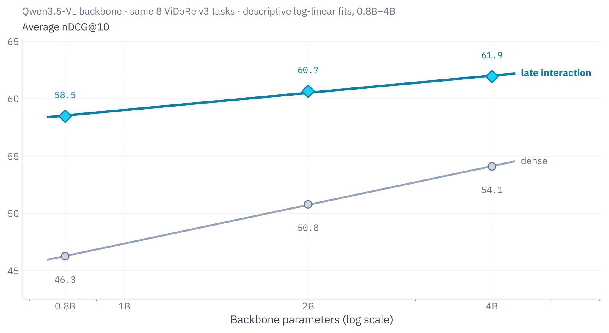
Page-level compression is a pressure point
Our own experiments. Teasing a future release!
Qwen3.5-VL backbone · same 8 ViDoRe v3 tasks · descriptive log-linear fits, 0.8B-4B
A teaser for a future release: we've been seeing the same thing in a project we're working on. We're training retrievers on the same backbone, Qwen3.5, with the same data recipes.
After pushing the dense limit higher and higher, we tried the same thing with late interaction, and the gap is quite telling again.
Spend the vector budget where evidence lives
On code, token merging still beats token pruning at every equal budget.
LateOn-Code · CoIR · % of baseline nDCG@10
LateOn-Code on CoIR
Hierarchical pooling holds ~91% of baseline NDCG@10 at just 20% of the vectors . Attention pooling falls to 2nd best.
The best pooling method varies by domain : the operational rule beats the method name. Experiment, and always measure.
A Brief Comparison of Training-Free Multi-Vector Sequence Compression Methods · Jha et al., 2026
The same paper also evaluated these strategies on code retrieval, on the CoIR benchmark. Again, pruning methods are inferior to pooling methods, and again we keep more than 90% of the retrieval quality at 20% of the index size.
Interestingly, here the ranking of pooling methods is flipped. The lesson: the exact best pooling method can vary by domain, so the method name is less important than the operational rule: we CAN pool token vectors together, but experiment with different methods, and always measure.
Merging beats deleting patches
In vision, sequence length becomes patch count . Again, deleting patches is brittle; merging similar patches keeps every region represented.
Semantic clustering · ColQwen2 · ViDoRe (v1) · % of baseline nDCG@5
Query-agnostic deletion can remove the one patch a future query needs .
Towards Storage-Efficient Visual Document Retrieval: Reducing Patch-Level Embeddings · Ma et al., 2025
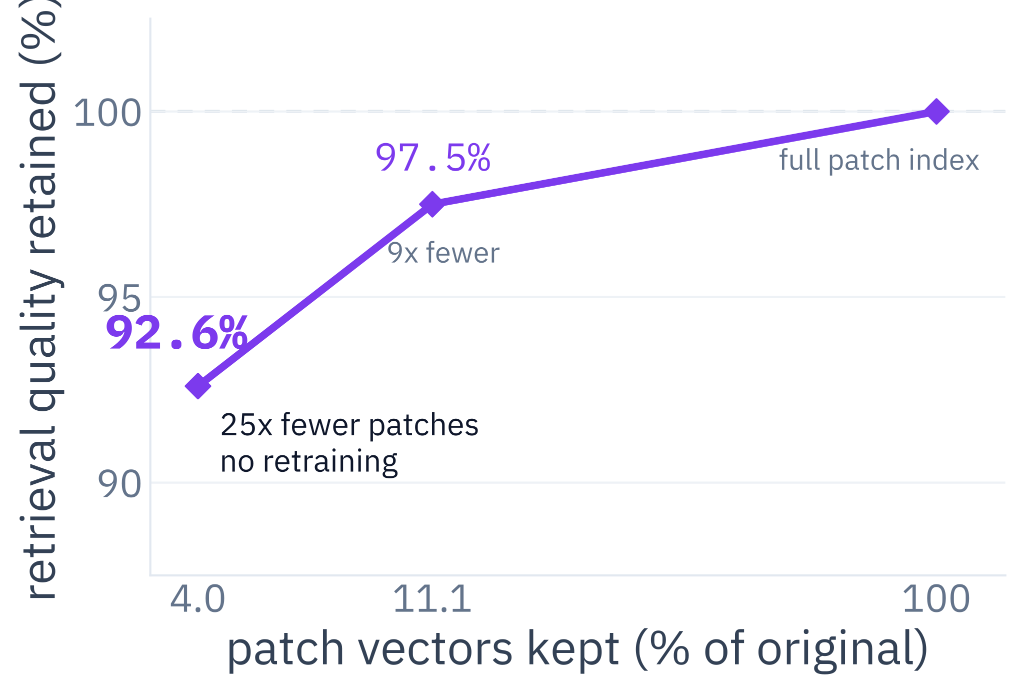
For vision, sequence length becomes patch count, and the same pattern appears: pruning is inferior to merging, and merging retains the lion's share of performance. Semantic clustering on the official ColQwen2 checkpoint retains 97.5% of baseline NDCG@5 at factor 9 and 92.6% at factor 25.
Clustering merges similar patch vectors while leaving every region represented; pruning has to happen without knowing the query, and query-agnostic deletion can remove the one patch a future query needs.
Post-hoc approaches aren't perfect, but we're getting there
Plug a recent model into MUVERA or SMVE and quality can collapse when geometry isn't friendly . But the fix already exists!
Full MaxSim (no shortcut, the target)
nDCG@10, exact scoring everywhere: the quality ceiling
MUVERA / SMVE w/ off-the-shelf model
the index builds fine, retrieval quality collapses!
The fix: a model trained for the index
LateOn-regularized, within 3 points of exact
What this means in practice
Some methods may seem too good to be true, and they aren't, to some extent! But they can be trained for.
Party is over: regularizing ColBERT models to fix efficient ANN methods · Chaffin, 2026
A short note: post-hoc methods such as MUVERA or SMVE share a hidden assumption: that the geometry of the token vectors is friendly, that is, well distributed in space. Many modern models are not: their token embeddings huddle in a narrow cone, so projections stop separating documents. The symptom is nasty because it is silent: the index builds, nothing errors, and quality collapses. Off the shelf, MUVERA scores 15.9 NDCG@10 where exact MaxSim scores 55.3. If you hit this, suspect the model before your pipeline.
Fixes come in steps: mean-centering at serving time recovers most of the gap, and training the model with the projection in the loop closes it to within three points. The message for practitioners: this failure is a model property, it is fixable at training time, and I expect models to increasingly ship index-aware.
My index is not static
Efficient late-interaction retrieval gets harder when the corpus changes .
01 Write amplification One document means many vectors; every insert, update, and delete costs more.
02 Assignment staleness New tokens may still be assigned to old centroids or codebooks.
03 Quality drift Monitor recall and assignment error; rebuild when thresholds cross.
New document
Index size < 1,000?
Full rebuild
Assign to nearest centroid
document is always retrievable
Distance < threshold?
Done
Add to buffer assignment kept meanwhile
Buffer < 100 docs?
Wait
Recluster & expand new centroids join the codebook
YES
YES
YES
NO
NO
NO
The practical pattern: write fast, search the buffer immediately, and rebuild deliberately . Systems such as NextPlaid make this lifecycle explicit.
One objection I hear less, but that may come to you: updates are a real complication. One document may mean around a hundred token vectors, so every insert, update, or delete has write amplification. Compressed indexes rely on centroids or codebooks learned from a snapshot; as the corpus changes, new tokens may fit those old assignments poorly and recall can drift without an obvious error.
A practical pattern: a small mutable buffer for new documents, immediate assignment to existing centroids when possible, and periodic reclustering or rebuilding once size, distance, or quality thresholds are crossed. The thresholds are illustrative; the monitoring principle is the part to keep.